Assumptions Under Which The OLS Estimators are BLUE
An Ordinary Least Squares (OLS) linear regression is one of the most common and widely used techniques in empirical research. In a nutshell, an OLS linear regression relates an outcome Y to a independent variable X by minimizing the sum of squared errors. The errors are essentially the differences between the observed outcomes and the outcomes that we predicted using X.
The reason why the OLS linear regression has had such a large impact on research likely lies in its simplicity and its desirable properties. Namely, the Gauss-Markov theorem states that—under certain assumptions—the OLS estimator is BLUE: the Best Linear Unbiased Estimator, a linear unbiased estimator with the lowest sampling variance. So, the expected value of the OLS estimate you obtain in a given sample are actually equal to the estimates of the entire population (unbiased). And what is more, the OLS estimate also varies less throughout the samples than all other linear unbiased estimators (best).
So what are the assumptions under which the OLS estimator is BLUE? This is not an easy question to answer because there have been many reformulations and extensions of the Gauss-Markov theorem over the years. In addition, many assumptions have different names in different disciplines, but actually mean the same thing. In what follows, we will try to provide an exhaustive list of the assumptions, although all the exposition including the original notation will be simplified for the general reader.
Let’s start with the earliest formulation by Carl Friedrich Gauss in 1821. Gauss’ paper was written in Latin, but was later translated to French by Joseph Bertrand in 1855. Gauss considered a linear additive model of the form:
Yi = β0 + β1X1i + β2X2i + … + βkXki + εi
- Linearity in parameters. Technically, this is not an assumption Gauss made explicitly, but he did start from the above model which is indeed linear in parameters. Another formulation of this assumption that means the same thing—but that is difficult to explain without matrix algebra—is that the -parameters are a linear function of Y. What this assumption means is that the -parameters enter the model linearly, they cannot be squared, cubed, or in logarithmic form, they cannot be multiplied with each other etc. This, however, does not mean that the X-variables have to be linear. For instance, the following models are linear in the parameters, but not linear in X:
Yi = β0 + β1Xi1 + β2X2i2 + β3X3i3 + εi
Yi = β0 + β1lnXi1 + β2lnXi2 + εi
Yi = β0 + β1Xi1 + β2Xi2 + β3Xi1Xi2 + εi
This model, however, is neither linear in the parameters nor in X:
Yi = β0Xβ1i1Xβ2i2εi
Note, however, that we can make the above model linear in the parameters, by taking the logarithm of both sides. We then get:
lnYi = lnβ0 + β1lnXi1 + β2lnXi2 + εi
This model is still nonlinear in parameter 0, but we can then estimate different parameters α0=lnβ0, α1=β1, and α2=β3. We then get:
lnYi = α0 + α1lnXi1 + α2lnXi2 + εi
It should be noted, however, that the parameters that minimize the sum of squared errors of the transformed equation do not necessarily minimize the sum of squared errors of the original equation.
- X-variables are fixed in repeated samples. As above, this is not an assumption Gauss made explicitly, but his formulation indirectly suggests this. This means that the X-variables are not random and observable (by extension, -parameters are not random but unobservable). We can choose their values, and we can set their values to be equal in each sample we take. For instance, if we conduct an experiment on the effect of gym training on health, we can divide people into a group that trains 2 hours (X=2), 1 hour (X=1), 30 mins (X=0.5), and no hours in the gym (X=0). We can set these four groups in each sample of people we take. On the other hand, the errors are random and unobservable.
- The errors are independently and identically distributed with an expected value of zero and a constant variance. Mathematically, this is expressed as i~iid(0,2). This assumption is the most confusing one, because it is often shortened to ‘independence’ leading to the rest of the asummption erroneously being forgotten. Essentially, this assumption indicates that the error terms have an expected value of zero, and the variance does not vary in the cross section (at one point in time) and also does not vary throughout time. Namely, this assumption consists of three different assumptions (although mathematically, the i.i.d. assumption is stronger than these three assumptions separately):
- The expected value of the error term in the population is zero. Mathematically, this can be expressed as E(εi) = 0. Intuitively, this means that the variables we unobserve, and are therefore in the error term, e.g., motivation or personality, may affect our outcome, but the effects of all these unobserved variables counteract each other so that the mean effect is zero.
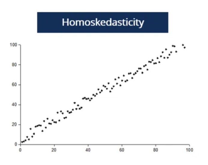
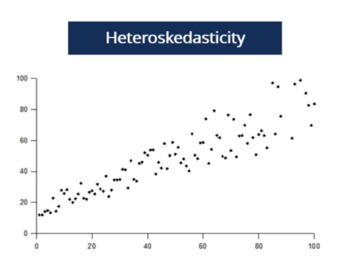
- Homoscedasticity. Mathematically, Var(εi) = 2 for all i and α2 < ∞. Intuitively, this means that the variance is constant in the cross section and finite (not infinite), or said otherwise, constant at one point in time. If you take different values of X, the variance in Y does not change. If this is not the case, and the assumption is violated, we speak of heteroscedasticity. For instance, consider the effect of education (X) on earnings (Y). People with only high school are likely to vary in earnings a lot. Some may be working for a minimum wage, while others are successful entrepreneurs. On the other hand, people with a Ph.D. are not as likely to vary in earnings as most of them will be earning high wages. It is unlikely for workers with a Ph.D. to be unemployed or to earn minimum wage. Hence, the variance will be higher for low levels of education than for high levels of education, leading to a violation of the homoscedasticity assumption.


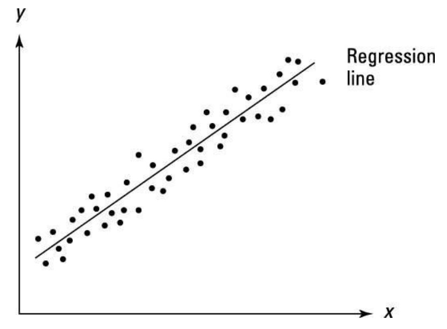
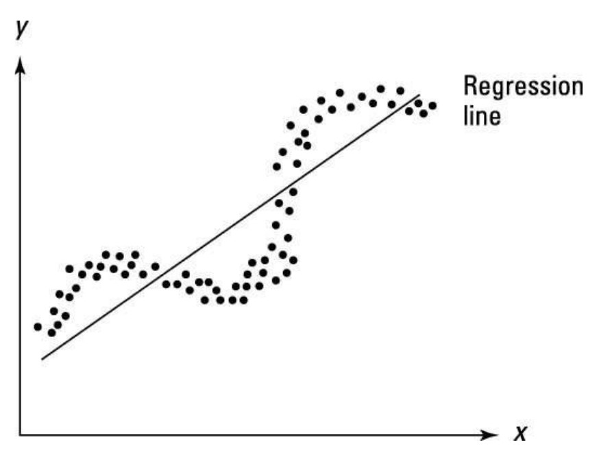
- No autocorrelation. Also referred to as ‘no serial correlation’. Mathematically, Cov(εi, εj) = 0 for i ≠ j. Intuitively, this means that the variance is constant over time. Said otherwise, the errors are uncorrelated meaning that the past value of an outcome should not provide information about the current value of the outcome. For instance, there is likely to be autocorrelation in earnings as an individual is unlikely to change their earnings over a short interval. In this case, the assumption of no autocorrelation would be violated. An example of no autocorrelation and autocorrelation is plotted on the figures below.
No autocorrelation

Autocorrelation

- Normally distributed error terms. Thus, the errors can be represented in a Bell-shaped curve. Intuitively, this means that most errors cluster toward the middle of the range of values, whereas the rest of the errors taper off symmetrically toward the extremes. So about 68.2% of the errors will be within one standard deviation around the mean and about 95.4% within two standard deviations.
- Linearity in parameters.
- X-variables are fixed in repeated samples.
- The expected value of the error term in the population is zero.
- Homoscedasticity.
- No autocorrelation.
As above, the first two assumptions were not explicitly mentioned by Markov, but his formulation indirectly suggests this. Note that the Gauss-Markov assumptions correspond to the Gauss assumptions, with the exception of the normality assumption that has been relaxed.
- Linearity in parameters.
- Strict exogeneity. Mathematically, E(εi | X1i, X2i) = 0. This is merely an extention of the assumption that the expected value of the error term in the population is zero, namely E(εi) =0. It should be noted, however, that having the expected value of the error term to be zero is less strong than having the expected value of the error term conditional on X-variables to be zero. Namely, it can be shown that if E(εi | X1i, X2i) = 0, then E(εi) =0, but not vice versa.
- Full rank. The name of this assumption comes from matrix algebra. Essentially, it assumes that there is no perfect multicollinearity. This means that the X-variables should not have a correlation of 1. Note that only perfect multicollinearity violates this assumption, the X-variables can be correlated as long as the correlation between them is not 1.
- Spherical errors. Again, the name of this assumption comes from matrix algebra. Essentially, this assumption means that the errors should be homoscedastic and that there should be no autocorrelation.
Under the above assumptions, the OLS estimator is BLUE, meaning the unbiased linear estimator with the lowest variance. The requirement that the OLS estimator is unbiased cannot be relaxed, because there are biased estimators with a lower variance, e.g., ridge regression. A significant recent development came in 2022, when Bruce Hansen tried to relax the assumption of linearity, saying that the OLS estimator is actually BUE: the best unbiased estimator. However, Stephen Portnoy showed that there are actually no unbiased estimators that are not linear. So saying that the OLS estimator is BUE is actually saying that the OLS estimator is BLUE as all nonlinear estimators will be biased.

Master the Science of Causal Inference
Latest Statistics Insights

Demystifying Degrees of Freedom
Demystifying Degrees of Freedom When doing hypothesis testing, everyone has encountered tests that depend on the so-called ‘degrees of freedom’. However, explanations of what degrees of freedom actually mean are lacking from most textbooks, and if they exist, these explanations are highly formulaic and lack intuition. Indeed, the phrase ‘degrees

Two-Sided vs One-Sided Hypothesis Tests: A Cautionary Tale
Two-Sided vs One-Sided Hypothesis Tests: A Cautionary Tale Hypothesis testing is a fundamental concept in statistics used to make decisions about populations based on sample data. When conducting hypothesis tests, researchers often have two options: one-sided and two-sided tests. In this blog, we’ll explore the differences between these two approaches